LightGBM Explained

LightGBM is probably the most widely used algorithm used for machine learning tasks on tabular data. On kaggle you almost always see it in the top 10 leaderboards, yet many (and I suspect most) only understand the interface of its official library, and not its technical underpinnings.

I recently implemented LightGBM from scratch in order to gain a better a technical understanding of it myself, however I couldn’t find any helpful resources besides the original paper online on the technicalities of LGBM, and so I decided I should write a blog post in order to help anyone on a similar endeavour in the future.

This post is intended for people with background knowledge in decision tree algorithms. If you don’t have any, I’d recommend watching some StatQuest videos on the topic or some independent reading and then coming back here to read the rest.

A Review of Gradient Boosted Trees

GBDT is an ensemble model of decision trees, which are trained in sequence. In each iteration, a new tree is constructed to predict the negative gradient (typically the residual error) of its previous prediction compared to a target value. By then adding this negative gradient (multiplied by a learning rate) to the previous output, its new prediction is moved closer to the target value, i.e. gradient descent.

The main cost in GBDT lies in learning the decision trees, and the most costly part of learning a decision tree is evaluating every possible split point that can be made across all features for maximum information gain.

Information Gain

The intuition is quite straight forward. Consider a simple example with 5 input/output pairs like the image below:

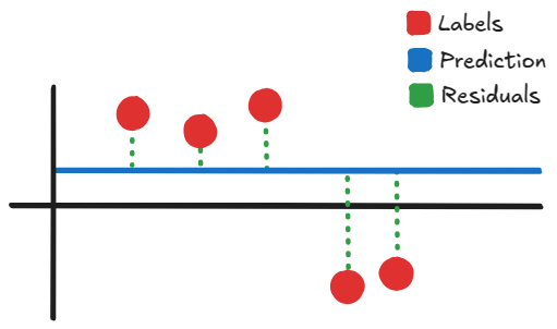
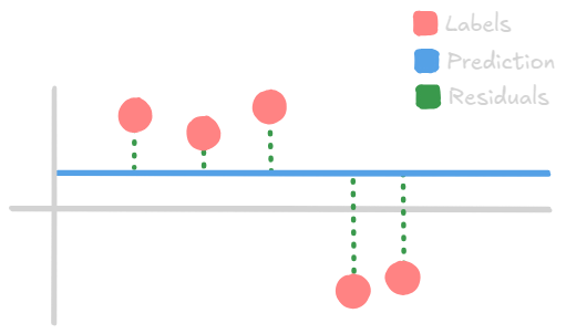Not drawn to scale

The initial prediction is just the average value of our datapoints’ labels. Our gradients (i.e. residuals) are the green dotted lines. What GBDT learns to do is predict the residuals and add the difference to the prediction, so that our final prediction might closer to our datapoints. The way it does this prediction is by splitting the data into separate “bins”, and adding the average residual within those bins to the initial prediction.

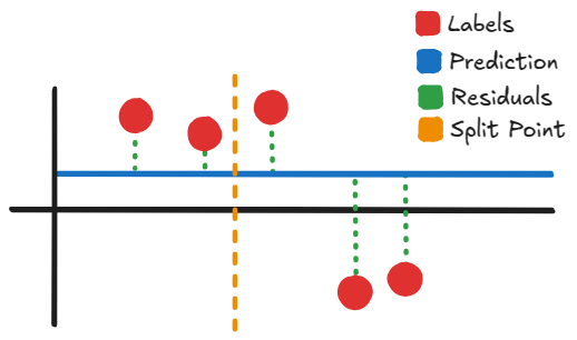
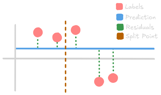
So for example with this split point here, the average of the left side’s residuals might be something like $-3$. While on the right side it could be $+6$. So then using this split point, whenever a data instance comes up to the left of it, it will add $+3$ to its current prediction, while if one comes up to the right it’ll add $-6$. (In reality we also multiply the residual by a learning rate, but that’s besides the point)

It’s not necessarily the case that what is being predicted is the residual of the model’s prediction. However, GBDT is typically evaluated using the loss function $\mathcal{L}(y, \hat{y}) = \frac{1}{2}(y - \hat{y})^2$, and so the gradients reduce to $\frac{\partial \mathcal{L}(y, \hat{y})}{\partial \hat{y}} = y - \hat{y}$. Although we could theoretically use any differentiable loss function and add its gradients as opposed to residuals.

You may have noticed though, that it’s not ideal for the data within a bin to be spread out (i.e. have high variance), as the average residual will end up far from any given data point. Therefore, we should have a way to quantify how good a split point candidate is. The most common gain metric uses the the normalized square of sum of residuals within its bin. This isn’t a direct measure of variance, but serves as a good proxy as if a bin contains a mix of positive and negative gradients, they’ll cancel out leaving us with small gain, while if the split does a good job at splitting negative/positive gradients then we’ll get a high gain value.

More formally, GBDT uses decision trees to learn a function from the input space $X^s$ into the gradient space $G$. Suppose we have a set with $n$ i.i.d. instances $\{x_1, \cdots, x_n \}$, where each $x_i$ is a vector with dimension $s$ in the space $X^s$. In each iteration of gradient boosting, the negative gradients (residuals) of the loss function with respect to the output of the model are denoted as $\{g_1, \cdots, g_n\}$. The decision tree model splits each node at the most informative feature (with the largest information gain). For GBDT, the information gain is usually measured by the variance after splitting which is defined below.

Definition 1. Let $O$ be the training dataset on a fixed node of the decision tree. The variance gain of splitting feature $j$ at point $d$ for this node is defined as

\[V_{j|O}(d) = \frac{1}{n_O} \left(\frac{(\sum_{\{ x_i \in O : x_{ij} \leq d \}} g_i)^2}{n^j_{l | O}(d)} + \frac{(\sum_{\{ x_i \in O : x_{ij} > d \}} g_i)^2}{n^j_{r | O}(d)} \right)\]

Where

\[\begin{align*} n_O &= \sum_{i} I[x_i \in O], \\ n^j_{l|O}(d) &= \sum_{i} I[x_i \in O : x_{ij} \leq d], \\ n^j_{r|O}(d) &= \sum_{i} I[x_i \in O : x_{ij} > d] \end{align*}\]

The two terms within the parentheses are the gains of the left and right child respectively. Because the denominators scale linearly with the number of data instances and the numerator scales quadratically, an additional division by $n_O$ is done in order to keep gain scale invariant.

For feature $j$, the decision tree algorithm selects $d^*_j = \operatorname{argmax}_d V_j(d)$ and calculates the largest gain $V_j(d^*_j)$. Then, the data is split according to the feature $j^*$ at point $d_{j^*}$ into the left and right child nodes.

Presorted GBDT Algorithm

One of the most popular algorithms for finding candidate split points within a dataset is the presorted algorithm, which for each feature, will sort them in increasing order, and uses the halfway point between adjacent elements as candidates. The time complexity for this is $\mathcal{O}(\text{#data} \times \text{#features})$.

Datasets can commonly have millions of rows and dozens of features, so this split point evaluation can get very costly!

Histogram-based GBDT Algorithm

Another popular algorithm is the histogram-based algorithm as shown for reference in Algorithm 1 of the LightGBM paper, where instead of finding split points along the sorted feature values, the histogram-based algorithm buckets continuous feature values into discrete bins which each contain an equal amount of samples (i.e. quantile binning) and uses these bins to construct histograms during training. The algorithm is presented below:

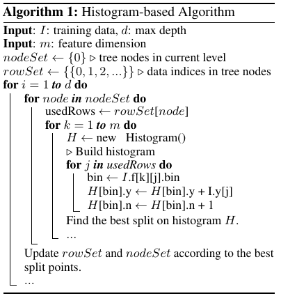
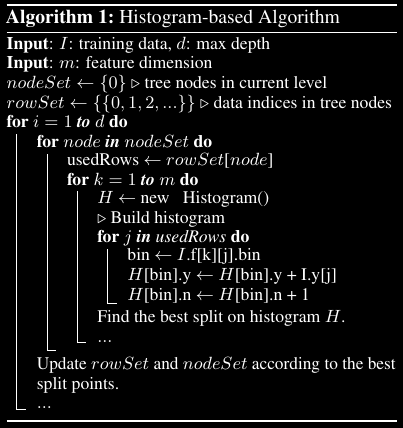
nodeSet contains pointers to the leaves in the current level. On the first iteration, the only node contained is the root which itself is a leaf, it averages the targets in the dataset to use as its prediction. The tree will grow level by level up to d times, at which point the max depth of the tree is reached and it will stop growing.

rowSet contains a mapping of nodes to data indices depending on whether or not the data points hold the criteria to end up at that node.

• For each node in nodeSet:
  • usedRows is assigned to the subset of the data that has a trajectory in the tree that lands at this node, which was precomputed and is found by indexing into rowSet with node.
  • For each feature k, we build a histogram:
    • Declare a new variable H and initialize it to an empty histogram.
    • For each sample j in usedRows, we populate the histogram:
      • Get the bin index for feature k on sample j and store it in bin, i.e., bin ← I.f[k][j].bin.
      • Increase the total sum of accumulated gradients within this bin - H[bin].y - by the gradient of the current sample, I.y[j].
    • Find the best split point on k. Just like how split points were found previously for candidates at individual samples, we do it now at the border of histogram bins.
  • Update rowSet and nodeSet according to the best split point across all features, and continue to the next iteration.

It costs $\mathcal{O}(\text{#data} \times \text{#features})$ for histogram building and $\mathcal{O}(\text{#bins} \times \text{#features})$ for split point finding. Since $\text{#bins}$ is usually much smaller than $\text{#data}$, histogram building will dominate the computational complexity. If we can reduce $\text{#data}$ or $\text{#features}$, it’ll substantially speed up the training of GBDT.

The large-scale datasets used in real world applications are typically quite sparse. GBDT with the pre-sorted algorithm can take advantage of this to reduce its training cost by simply ignoring the features with zero values. However, GBDT with the histogram-based algorithm cannot take advantage of this sparse property as it needs to retrieve feature bin values for each data point no matter if the feature value is zero or not. It would be great if the GBDT with the histogram-based algorithm could take advantage of this sparsity as well.

To address this, the authors introduce Gradient-based One-Side Sampling (GOSS) and Exclusive Feature Bundling (EFB).

Gradient-based One-Side Sampling

The point of GOSS is to reduce $\text{#data}$ . It works by simply ignoring data instances whose previous gradients (AKA residuals) were small, the reasoning being that data instances with small gradients are already well trained and don’t need to be focused on. The only problem with this is that ignoring these instances will shift the data distribution and can cause the model to overfit to the new distribution, while “forgetting” what it knew of previous data instances.

To address this GOSS keeps all the instances with large gradients and performs random sampling on the instances with small gradients. In order to compensate for the influence to the distribution, when computing information gain, GOSS introduces a constant multiplier for the data instances with small gradients. Specifically GOSS first sorts the data according to the absolute value of their gradients, and selects the first $a \times 100\%$ instances. Then it randomly samples $b \times 100\%$ instances from the rest of the data. GOSS then amplifies the lower gradient samples by $\frac{1-a}{b}$ when calculating information gain. This allows to put more focus on under-trained instances without changing the original data distribution by much.

$b$ is referring to the portion of the entire dataset to pull from the small gradient data, as a corollary, $b$ is bounded by $1-a$.

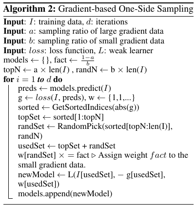
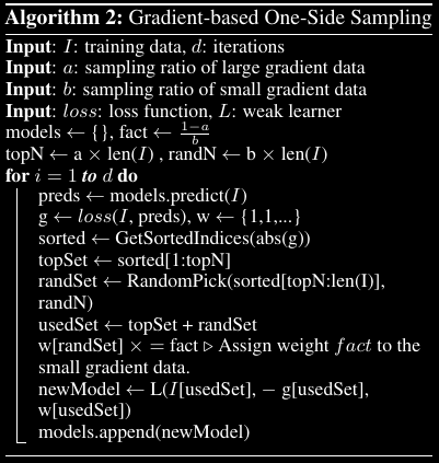
The statements before the loop are obvious. We’re simply initializing a model object to an empty set, computing the constant fact for later, and calculating the topN and randN amounts based off our chosen $a$ and $b$. Within the loop we:

1. Get our current predictions from our model and store it in pred. In the first iteration our prediction is simply the average of our dataset. Subsequent iterations consist of the average plus the weighted sum of corrections that each tree predicts.

2. We calculate our gradients for each input and store it in g.

3. The weights w are initialized to a 1d vector of ones. (This will be used to apply the $\frac{1-a}{b}$ amplification described earlier)

4. We then sort the gradients by their absolute value, store the indices of the first topN of them into topSet, and store random set of indices of size randN from the rest of the gradients into randSet.

5. topSet and randSet are concatenated and stored in usedSet.

6. The weights whose indices are within randSet are assigned to fact, so that we can amplify the subset of weights that pertain to the lower valued distribution.

7. We then create a new weak learner which uses the histogram based algorithm described previously using our subset of gradients within usedSet.

Theoretical Analysis

As seen in the algorithm, training instances are first ranked according to the magnitude of their gradients in descending order. The top $a \times 100\%$ of gradients are kept and can be called the instance subset $A$. Then, for the remaining subset $A^c$ containg $(1-a) \times 100\%$ of instances with smaller gradients, another subset $B$ is taken as a random sample of $b \times 100\%$ of from the elements in $A^c$. Finally, the instances are split according to the estimated variance gain $\tilde{V}_j(d)$ over the subset $A \cup B$, i.e.,

\[\tilde{V}_j(d) = \frac{1}{n} \left( \frac{(\sum_{ x_i \in A_l } g_i + \frac{1-a}{b}\sum_{ x_i \in B_l } g_i)^2}{n^j_l(d)} + \frac{(\sum_{ x_i \in A_r } g_i + \frac{1-a}{b}\sum_{ x_i \in B_r } g_i)^2}{n^j_r(d)} \right)\]

Where

\[\begin{align*} A_l &= \{ x_i \in A : x_{ij} \leq d \} \\ A_r &= \{ x_i \in A : x_{ij} > d \} \\ B_l &= \{ x_i \in B : x_{ij} \leq d \} \\ B_r &= \{ x_i \in B : x_{ij} > d \} \\ \end{align*}\]

Notice this is just a variation on Definition 1., the only difference is that we break up the squared sum in each term into the sum of the large and small gradients, then multiply the small sum with $\frac{1-a}{b}$.

Thus in GOSS, only a subset of the gradients are used to compute the estimated $\tilde{V}_j(d)$, instead of the more accurate $V_j(d)$ which uses all instances to determine the split point. Because of this, the computation cost can be largely reduced.

Approximation Error

According to Ke et al. (2017) the following theorem indicates that GOSS will not lose much training accuracy and will outperform random sampling (as opposed to the weighted sampling using the largest gradients). They left the proof within the supplementary material, and I’ve omitted it as well as it doesn’t bring forward any intuition.

Theorem 2 The approximation error in GOSS is denoted as

\[\mathcal{E}(d) = |\tilde{V}_j(d) - V_j(d)|\]

and

\[\begin{align*} \bar{g}^j_l(d) &= \frac{\sum_{x_i \in (A \cup A^c)_l} |g_i|}{n^j_l(d)} \\ \bar{g}^j_r(d) &= \frac{\sum_{x_i \in (A \cup A^c)_r} |g_i|}{n^j_r(d)} \end{align*}\]

With probability $1 - \delta$ we have

\[\mathcal{E}(d) \leq C^2_{a, b} \ln 1/\delta \cdot \max\left\{\frac{1}{n^j_l(d)}, \frac{1}{n^j_r(d)}\right\} + 2DC_{a,b}\sqrt\frac{\ln 1/\delta}{n}\]

Where $C_{a,b} = \frac{1-a}{\sqrt{b}}\max_{x_i \in A^c}|g_i|$ and $D = \max(g^{-j}_l(d), g^{-j}_r(d)).$

So here $\delta$ would be the probability that the inequality does not hold. As we decrease $\delta$ (i.e., higher confidence), the bound increases. Furthermore, there are two things which can be said about the inequality:

1. The approximation error of GOSS asymptotically decreases with $\mathcal{O\left(\frac{1}{n^j_l(d)} + \frac{1}{n^j_r(d)} + \frac{1}{\sqrt{n}}\right)}$. $\frac{1}{n^j_l(d)}$ and $\frac{1}{n^j_r(d)}$ come from the $\max$ operation in the first term of the inequality, while the $\frac{1}{\sqrt{n}}$ comes from the second term of the inequality. If the split is well balanced, (i.e., $n^j_l \geq \mathcal{O}(\sqrt{n})$ and $n^j_r \geq \mathcal{O}(\sqrt{n})$), then the approximation error will be dominated by the second term of the inequality, which reduces to 0 in $\mathcal{O}(\sqrt{n})$ with $n \rightarrow \infty$. Which means that when we have a lot of data, the approximation is quite accurate.

2. Random sampling is a special case of GOSS with $a = 0$. In many cases, GOSS could outperform random sampling, under the condition $C_{0, \beta} > C_{a, \beta-a}$, which is equivalent to $\frac{\alpha_a}{\sqrt{\beta}} > \frac{1 - a}{\sqrt{\beta - a}}$ with $\alpha_a = \max_{x_i \in A \cup A^c} |g_i| / \max_{x_i \in A^c} | g_i |$. Intuitively, random sampling would perform worse as we’d receive a weaker signal from the gradient data than when using $a > 0$.

Generalization Performance

Since our training data is only a finite sample from the unknown underlying data distribution, we’d like to analyze how well decisions made on this sample (i.e., split gains) generalize to the full, out-of-sample distribution.

We consider the generalization error in GOSS $\mathcal{E}^\text{GOSS}_\text{gen}(d) = |\tilde{V}_j(d) - V_*(d) |$, which is the gap between the variance gain calculated by the sampled training instances in GOSS and the true variance gain for the underlying distribution.

We can establish an upperbound on on $\mathcal{E}^\text{GOSS}_\text{gen}(d)$ which should be equal to the generalization error of $V_j(d)$ added to the approximation error of GOSS, more formally we have:

\[\mathcal{E}^\text{GOSS}_\text{gen} \leq \mathcal{E}_\text{gen}(d) + \mathcal{E}_\text{GOSS}(d) \triangleq |V_j(d) - V_*(d) | + |\tilde{V}_j(d) - V_j(d) |\]

Thus, the generalization error with GOSS will be close to that calculated using the full data instances if the GOSS approximation is accurate. On the other hand, sampling will increase the diversity of the base learners, which potentially help to improve generalization performance.

Exclusive Feature Bundling

If you recall from earlier, the two main bottlenecks in our GBDT algorithm using our histogram-based construction was $\text{#data}$ and $\text{#features}$. GOSS does a good job of reducing $\text{#data}$, however $\text{#features}$ can still be large. Exclusive Feature Bundling (EFB) reduces the total number of features within a dataset, by merging sparse features that rarely both show a non-zero value at the same time. In other words, if many columns almost always show zero, we can combine them into a single column in such a way that we can distinguish when a different feature is active.

The new merged features are called feature bundles, and constructing these bundles efficiently allows us to change our histogram building algorithm from $\mathcal{O}(\text{#data} \times \text{#features})$ to $\mathcal{O}(\text{#data} \times \text{#bundles})$, where $\text{#bundles} \ll \text{#features}$. And since the features are sparse we can do this almost losslessly, i.e., without hurting accuracy.

In order to bundle features, two problems must be addressed. The first is which features to bundle, and the second is how to merge them.

Bundling

The authors show it is NP-Hard to find the optimal bundling strategy, and that the problem can be reduced to that of the graph coloring problem (I won’t show the proof as its verbose and unnecessary for this blog post). They also state that randomly polluting a small fraction of feature values will affect the training accuracy by at most $\mathcal{O}([(1 - \gamma)n]^{-2/3})$ where $\gamma$ is the maximal conflict rate in each bundle. So if we choose a relatively small $\gamma$ we should be able to find a good balance between accuracy and efficiency. Keeping in mind that this is an instance of the graph coloring problem, the algorithm devised for greedy bundling is effectively a transfer of that one used for greedy coloring:

First we can construct a graph with weighted edges, which can be represented by an $F \times F$ adjacency matrix. The $i$th row corresponds to the $i$th feature, while the $j$th entry corresponds to the number of conflicts with the $j$th feature. We can calculate the total degree of a feature by summing along its row, and then sort each feature by their degree (in other words by the total amount of conflicts).

Then, for each feature in the ordered list, we can either assign it to a pre-existing bundle if the resulting conflicts within that bundle is small (threshold controlled by $\gamma$), or we can create a new bundle.

Below is the algorithm in its entirety:

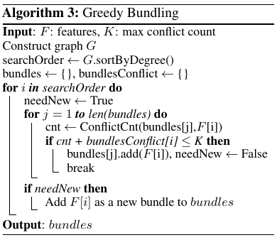
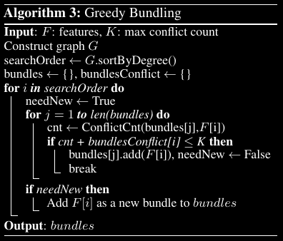
1. We first construct a graph the graph G. Each entry corresponding to the number of conflicts between the $i$th and $j$th feature.

2. We initialize searchOrder, which is a list of feature indices sorted by degree in G.

3. Initialize both bundles and bundlesConflict to an empty set.

4. For i in searchOrder:

   • initialize needNew to True.
   • for j in len(bundles) (looping through each bundle we already have):
     • initialize cnt to ConflictCnt(bundles[j], F[i]). This calculates how many new conflicts would be created in the bundle currently being looked at if we were to add feature i.
     • If cnt + bundlesConflict[i] <= K. K is the maximum permitted conflicts within a bundle calculated as $\gamma \times n$. However, there does seem to be a typo within the paper, adding cnt to bundlesConflict[i] doesn’t make sense, at least not from what I’ve interpreted. What would make much more sense is adding cnt to the jth entry in bundlesConflict, as we’d then be evaluating: if we add ith feature to the current bundle being looked at, then do we surpass our maximum threshold K? Which is the intention of the algorithm described in the paper.
       • Add the current feature to the bundle, set needNew to false, and break out of the loop.
       • It also seems that the algorithm as written in the paper has forgotten to update bundlesConflict, but it would make sense to do so here before breaking out the loop so that bundlesConflict[j] would reflect the new total conflicts with the ith feature included.
   • If needNew is true, which means our ith feature hasn’t been added to any bundle, then add a new bundle with only the ith feature as a member to bundles.

The time complexity of this algorithm would be $\mathcal{O}(\text{#features}^2)$ due to the graph construction and ordering, and it is only processed once before training. This time complexity is fine when the number of features aren’t very large, but in the case where there are millions of features to consider this can still be quite expensive.

Because of this the authors propose a different sorting method in which we simply choose the sort order by the number of non zero values a feature holds, as the more non-zero values a feature holds the more likely it is to conflict. The author’s didn’t include the new algorithm within the paper and neither will I, as its only difference to what was just discussed is that the ordering before the main loop is done differently.

Merging Features

For the second issue we must have an efficient way of merging features within a bundle in order to lower the overall training complexity. We need to ensure that the value of original features can be identified from the merged bundle. Since the histogram based algorithm already uses discrete bins to represent a feature as opposed to continuous values, we can simply concatenate the bins from different features within a bundle to merge them. That way, different features reside in different bins and we’re able to represent them within a single column.

For example, say we have two features $i$ and $j$ whose values reside in the discrete interval $[0, 5]$ and $[0, 10]$ respectively. Then the feature $k$ that is the merge of $i$ and $j$ will have values which reside in the range $[0, 15]$. If feature $i$ is non-zero then the value of $k$ will be between $[1, 5]$, if feature $j$ is non-zero then the value of $k$ will be between $[6, 15]$, and if both are non-zero (i.e. a conflict), then one of the original values will have to take precedence over the other, this is typically the last evaluated non-zero feature as is seen in the algorithm below:

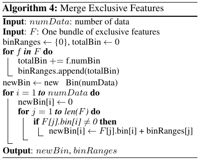
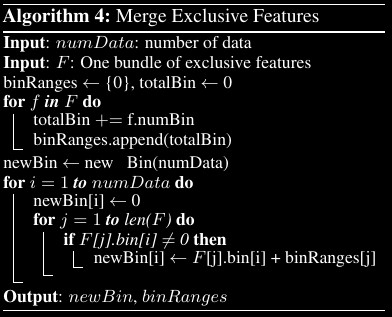
• Initialize binRanges to the set including 0. binRanges will include a prefix sum of the total amount of bins each feature includes, so that when merging, we can properly offset each feature to its correct range.
• InitializetotalBin to 0.
• For each feature in our feature bundle:
  • Increment totalBin by the number of bins the current feature includes.
  • Append totalBin to binRanges. (i.e. continue the prefix sum)
• We then initialize newBin to a new object of type Bin containing numData entries. The exact object used isn’t necessary, what’s important to know is that a new column is being created to replace our merged features, with a size of numData.
• For i = 1 to numData:
  • initialize newBin[i] to 0.
  • For each feature within the bundle
    • If our current feature is not equal to zero, then set newBin[i] to the current feature’s value offset by the total number of bins preceding it, which is calculated at binRanges[j].

Conclusion

And that’s everything! To recap, the novelty that LightGBM brings forth is:

• Gradient-based One-Side Sampling (GOSS), which allows us to reduce the number of samples used to evaluate split points

• Exclusive Feature Bundling (EFB), which permits us to merge sparse, mutually exclusive features, into a single dense feature, which reduces the complexity of evaluating split points.

I hope this blog post brought you some clarity as to how LightGBM works internally, if you have any questions or remarks feel free to leave a comment!

Thanks, Yanis

References

• Ke, G., Meng, Q., Finley, T., Wang, T., Chen, W., Ma, W., Ye, Q., & Liu, T.-Y. (2017). LightGBM: A highly efficient gradient boosting decision tree. Advances in Neural Information Processing Systems. Paper

• Ke, G., Meng, Q., Finley, T., Wang, T., Chen, W., Ma, W., Ye, Q., & Liu, T.-Y. (2017). LightGBM Supplementary Material. Advances in Neural Information Processing Systems. Supplemental

• Microsoft. (n.d.). Microsoft/LightGBM: A fast, distributed, high performance gradient boosting (GBT, GBDT, GBRT, GBM or Mart) framework based on decision tree algorithms, used for ranking, classification and many other machine learning tasks. GitHub